You can find source codes on this link.
Introduction
In numerical algorithms, matrices often represent real-world problems, as they are the most efficient tools for translating physical problems into computer language. An example of this is the 3D Heat Map, which can simulate heat flow, identifying potentially hazardous situations and suggesting improvements in materials. Undoubtedly, a 3D Heat Map can be beneficial in solving a variety of different problems.
Furthermore, solving Matrix Equations requires a dedicated method like a Matrix equation solver. In my project, I utilize the Conjugate Gradient method as my solver. This choice stems from the versatility of the Conjugate Gradient method, widely applicable across various fields, including AI.
In addition, I employed the Finite Difference Method to derive the A matrix, enabling me to elucidate the algorithm I’ve employed.
Algorithm of the Project
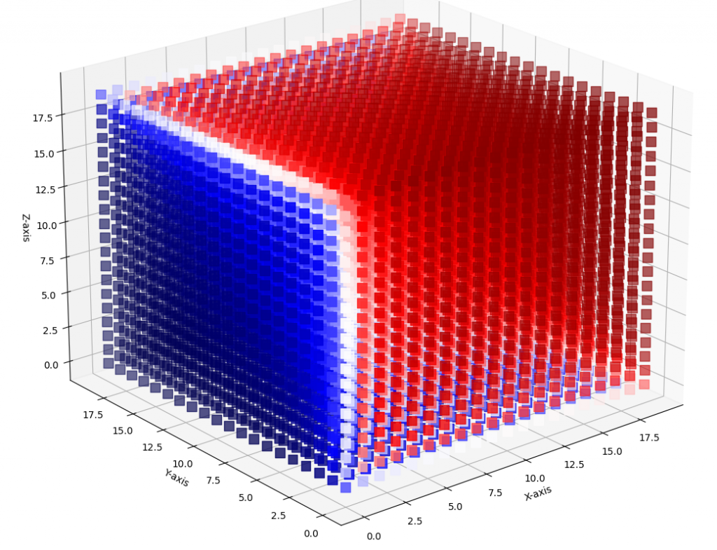
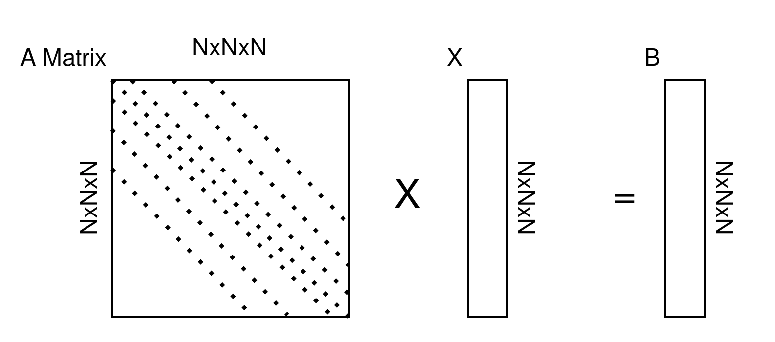
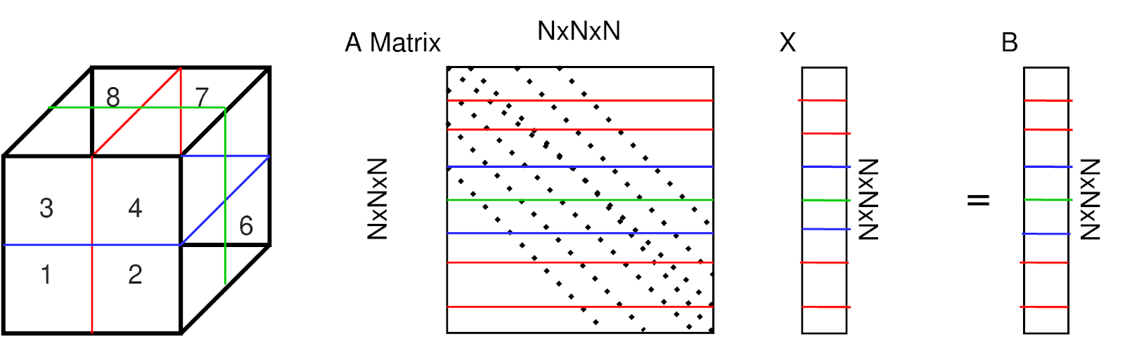
First of all, imagine a cube, this cube is heating each surface certain value. and you as a researcher want to find out the final heat distribution. You want to know the temperature values of the cube at equilibrium. Hence you need a Heat Map Equation which is “Ax=B”. To create A matrix, you need to know the finite difference method. A is stored finite-difference relationships to heat points information. For 3D Finite Difference, the Heat Equation is
K+ -6 T (x,y,z)+ T(x-1,y,z)+ T(x+1,y,z)+ T(x,y-1,z)+ T(x,y+1,z)+ T(x,y,z-1)+ T(x,y,z+1).
So, A matrix is a symmetric sparse seven-band matrix.
X keeps discrete heat points. B keeps surface heat values according to given surface heat values if the point is not located at the surface then B values become initialization heat values.
Of course, we do parallel processing so I have to divide all matrices and vectors into processes like the above.
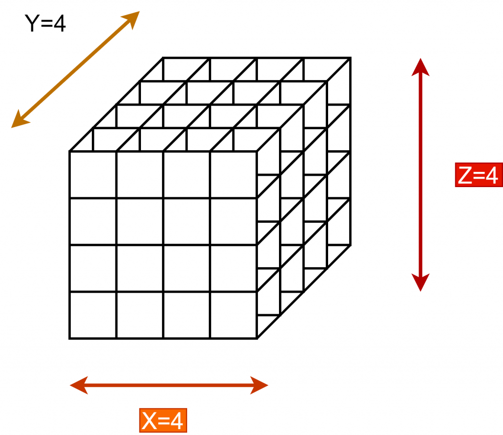
Thus, I separated the A matrix, X vector, and B vector row-based. I have separated the processors by creating a cartesian topology, with the processors numbered in cubes below. Of course, there will be ghost points due to separation. Processors whose surfaces are in contact with each other, when necessary, send data to each other, solving these ghost points problems.
I use MPI Cartesesan Shift to find the neighbors of each processor. Thus, I get the information of LEFT, RIGHT, FRONT, BACK, BOTTOM, and TOP processors.
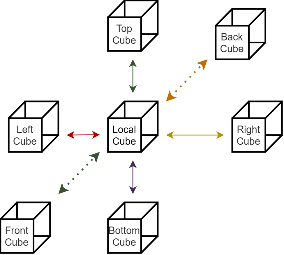
I created 3 different contiguous types for this communication. These are XZ_TYPE, XY_TYPE, and YZ_TYPE.
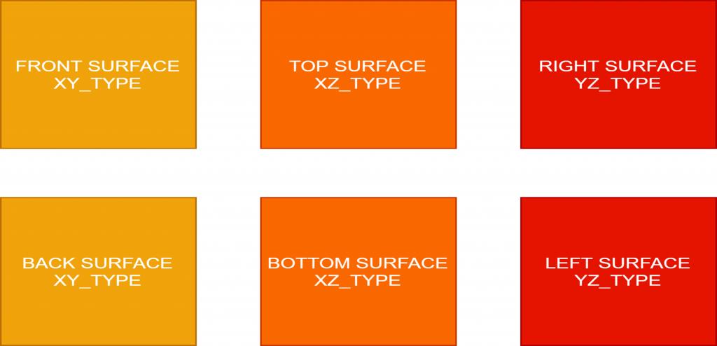
Thus, I receive and send data with these special data types according to the relevant surface.
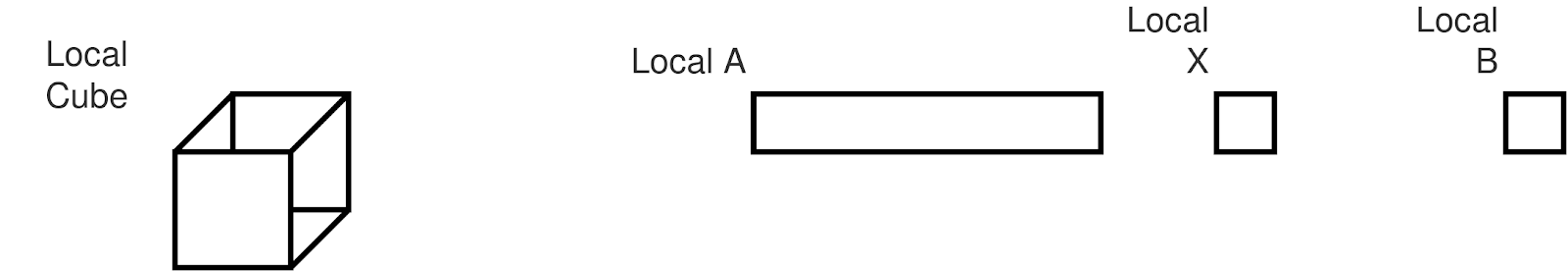
You can see the data in the local of each processor in the figure below.
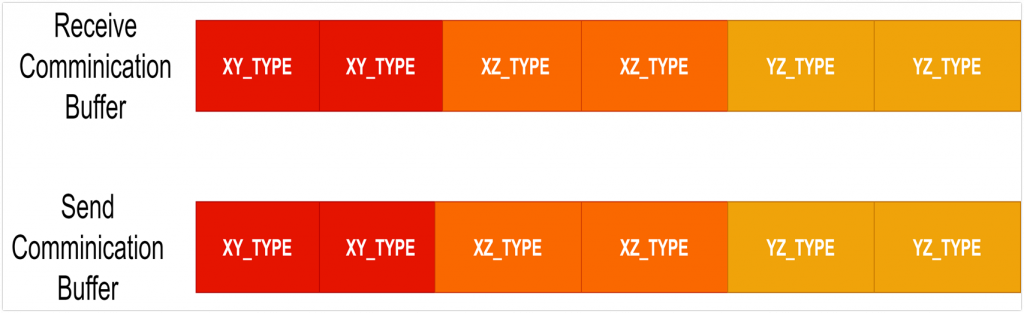
Now let’s talk about the two buffers I need to send and receive ghost points. I use one of these buffers to receive and the other to send. Each buffer is divided into 6 parts, each of these 6 parts is designed to hold data on a surface. Send buffer is used to send local surface points. As expected, Receive is used to receive ghost points in its neighbors. so I solve my processes with ghost point thanks to these buffers. MPI_Isend and MPI_Recv functions are used when sending and receiving these buffers.
Therefore, I created all fundamental matrices and vectors to start solving the Heat Equation.
Conjugate Gradient Descent
After the above operations, it remains to solve the equation in this step. As I said before, I solved this equation using the Conjugate Gradient method. You can see the Conjugate Gradient method’s main algorithm in the figure below.
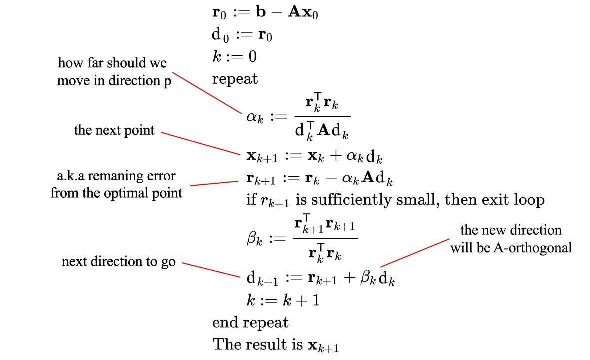
The main idea behind the Conjugate Gradient method is to find the global minimum, that is, the solution point, by following the slopes in the equation space. Therefore, the X vector is given a random value and the algorithm is stopped when the error value falls below a certain tolerance value by updating it iteratively with Alpha (Distance amount), and Beta (Direction) values.
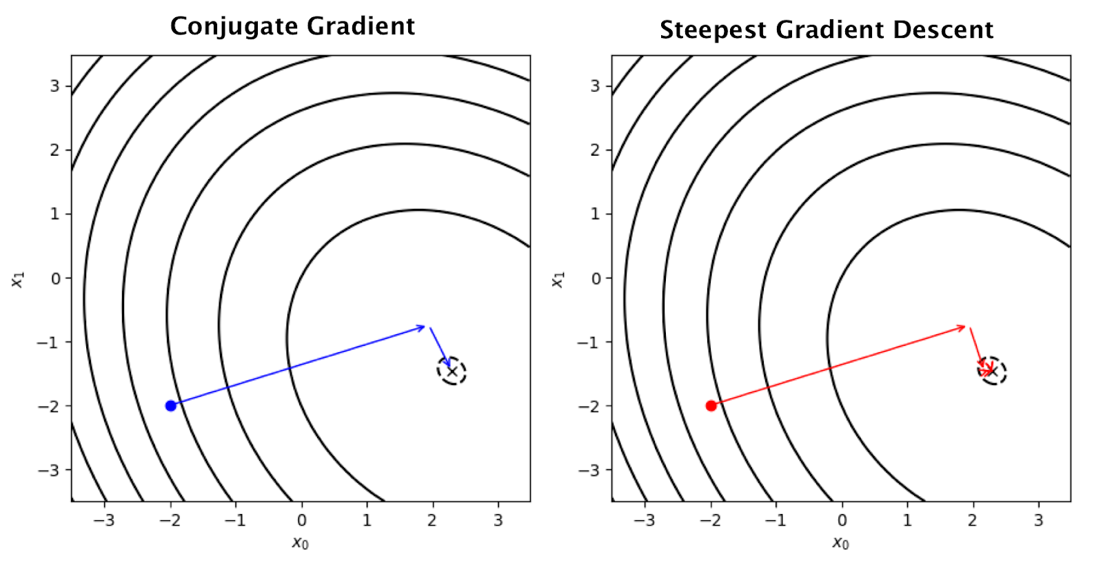
In the figure below, the blue dot represents the random starting point. Then, by applying the gradient descent algorithm, it is shown how the two steps converge to the X point.
Alpha and Beta are two very important values. And to get them, I need to add the local Alpha and Beta values obtained on all processors. So, I used the MPI_AllReduce algorithm. Because of this, all my processors need to be synchronized in certain places, which of course creates a communication overhead.
Conjugate Gradient Method With MPI
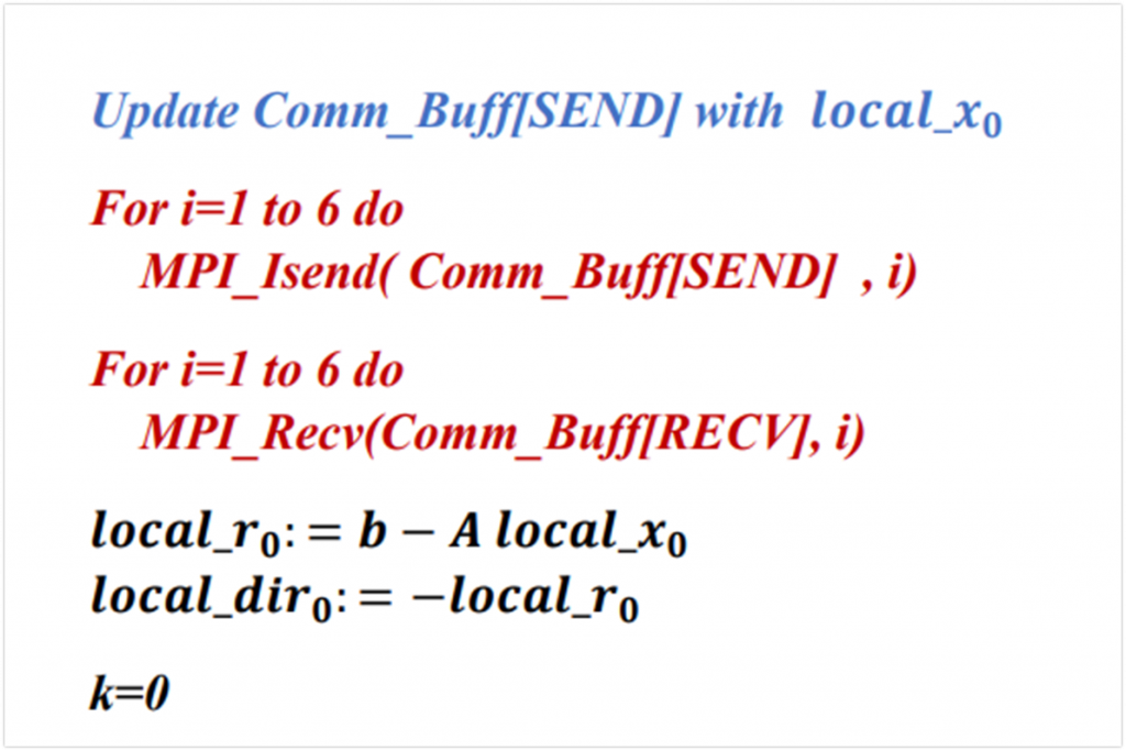
Now we can pass the Conjugate Gradient Method. At the start of the Conjugate Gradient Method, they will send and receive points on the surface of local x0 values to all neighboring processors. That’s why I’m updating the Send Comm Buff. then I update the Local residual and local direction vectors as you can see. I have initialized the Conjugate Gradient Method.
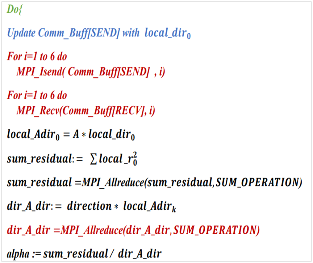
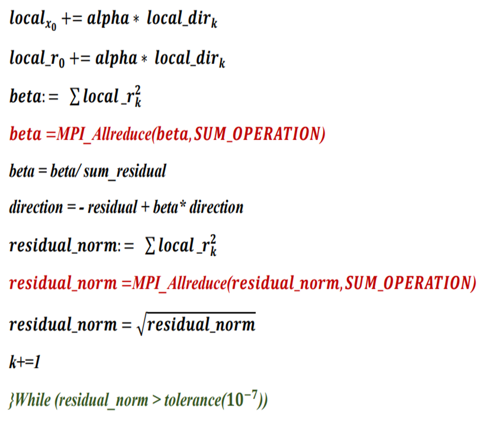
We’ve come to the main part. Here we have a do-while loop that will continue until our error is below 10^-7. 10^-7 I chose it. This may change according to the desired tolerance value. The local_direction vector is the most important thing in the Conjugate gradient method. because we update the local x vector according to this direction method and take one more step towards a more accurate result. Therefore, at the beginning of each iteration, we update the ghost points with neighboring processors and calculate the next local dir. To calculate the alpha value, which is another important parameter, I had to sum the local residual squares and add them with MPI_Allreduce and values from all other processors. After obtaining the alpha value, I updated the local x and local residual vectors. then I first do the sum of the square of the local_residu and the vector in the local to get the Beta value. Then I get the beta value by adding the beta values in all other processors with the MPI_ALLreduce function. So I update the direction vector. then again using MPI_ALLreduce I get the residual norm value. and I’m rooting it and comparing the tolerance value. I decide whether to continue or not depending on the situation.
Results
Core size: 1, 8, 16, 32, 64, 128, 224
N is 224 , N^3 = 11239424
I chose a cube with the size of 224*224*244 as the Test number. Thus, I got the A matrix dimension of 224^3 x 224^3. I tried larger numbers but couldn’t get an accurate result due to a server issue. Below you can see the result graphs in order.
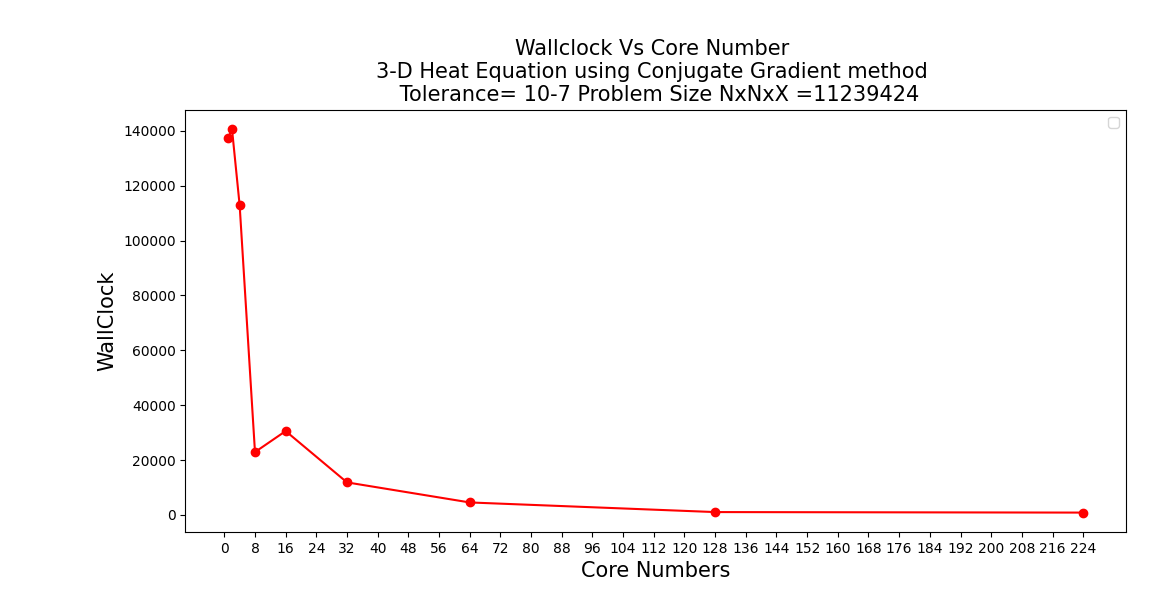
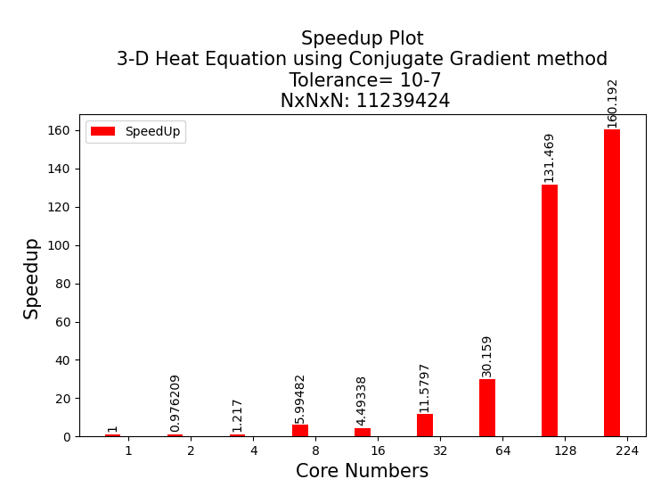
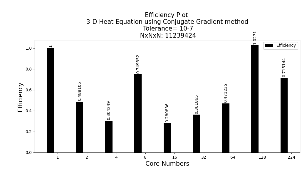
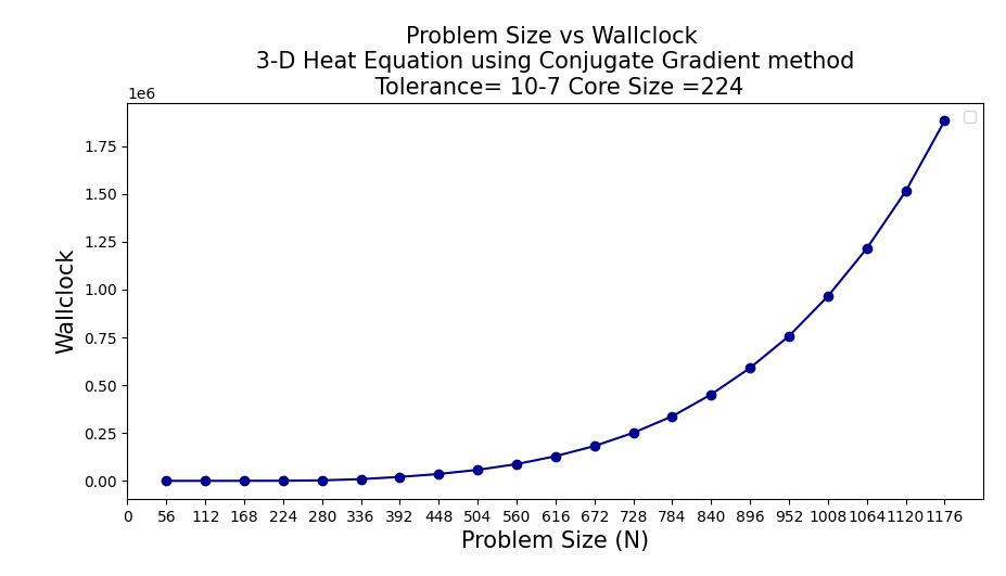
According to the results I obtained above, I am not getting good enough results compared to the normal single processor, where I use a small number of processors. I think this is because of the communication overload. An almost exponential increase is observed as the number of cores increases. The model with 128 cores gives the best result in the efficiency plot. I attribute this to the fact that it is 128 2^7. Thus, I think the Communication overload will be lower (Bufferfly communication). I would test this if the server system allowed me to use 256 cores. Other than that, the Problem size vs Wall Clock figure gives exactly the N^3 graph, which is the result we expected.
Potential Limits and Enhancements
First of all, if I need to talk about the potential limits, of course, hardware limitations can limit the working speed. Because data transfer between processors is a limiting factor. Apart from that, the frequency and cache size of the processors directly affect it. In terms of software, I tried to make MPI communication blocks async as much as I could. But I couldn’t make AllReduce and MPI_Receive side async. Apart from these, some MPI_Vector data types instead of MPI_Continguous data types could have enabled me to transfer my data more effectively. In general, I can say that these are the main factors limiting my limits.
How to Improve My Result
Design an algorithm that decreases communication to other cores,
Try to bigger matrix size than 224
Try to optimize the Conjugate gradient method better
Conclusion
I learned a lot from this project. I learned how to create both Heat Map problems and how to solve this problem with the Conjugate Gradient method. Apart from that, I learned how to set up parallel processing and MPI, which is the main topic of the course. I learned how to apply it, even if I didn’t fully implement it in the best way. I am very happy to work on such a project.
İlk Yorumu Siz Yapın